Google Play store Exploratory Data Analysis using Python

Exploratory Data Analysis (EDA) is a fundamental step in the data analysis process, focusing on summarizing and visualizing the main characteristics of a dataset. The primary goal of EDA is to gain insights into the data, detect patterns, identify anomalies, test hypotheses, and check assumptions. This process is crucial before applying more complex statistical methods or machine learning algorithms.

Why EDA?

• Understand Data Structure: Gain insights into the data’s organization and the types of variables present.
• Identify Patterns: Discover trends and relationships between variables.
• Detect Anomalies: Spot outliers or unusual data points that may require further investigation.
• Assess Assumptions: Evaluate the validity of assumptions for statistical modeling.

Introduction

The Google Play Store is a digital distribution service developed by Google, serving as the official app store for Android smartphones and tablets. For Android users, it is by far the most popular and convenient platform for discovering new apps and other digital content. As of February 2017, the repository offers more than 2.7 million Android apps and over 40 million songs. Whether you’re looking for movies, music, magazines, or e-books, Android users are most likely to find it on the Google Play Store.

To access this vast content, Android users rely on the Google Play Store app, which was introduced in March 2012 after Google merged its Android Market and Google Music services into a single unified platform. Non-Android users can still access content directly through the Google Play website.

About Project

Today, 1.85 million different apps are available for users to download. Android users have even more from which to choose, with 2.56 million available through the Google Play Store. These apps have come to play a huge role in the way we live our lives today.

The Objective of this Analysis is to find the Most Popular Category, find the App with largest number of installs, the App with largest size etc.

• The data consists of 20 column and 10841 rows.

Before diving into the steps of Exploratory Data Analysis (EDA), it’s essential to set up your Python environment. Here’s a streamlined guide to get you started:

1. Download and Install Anaconda:

• Visit the Anaconda Download Page: Navigate to the Anaconda Distribution download page.
• Select the Appropriate Installer: Choose the installer that matches your operating system (Windows, macOS, or Linux).
• Download and Install: Click on the “Download” button, then run the installer and follow the on-screen instructions.

Note: During installation, you can opt to add Anaconda to your system’s PATH environment variable. This step ensures that Anaconda’s executables are accessible from the command line.

2. Download and Install Visual Studio Code (VS Code):

• Visit the VS Code Download Page: Go to the Visual Studio Code download page.
• Select the Appropriate Installer: Choose the installer that matches your operating system.
• Download and Install: Click on the “Download” button, then run the installer and follow the on-screen instructions.
• Note: Ensure that you select the option to add VS Code to your system’s PATH during installation. This allows you to open VS Code from the command line using the code command.

3. Create a Virtual Environment:

• Creating a virtual environment helps manage project-specific dependencies and prevents conflicts between packages.
• Open Anaconda Prompt: Launch the Anaconda Prompt from the Start Menu (Windows) or Terminal (macOS/Linux).
• Create the Virtual Environment: Run the following command to create a new environment named venv with Python 3.12:

conda create -p venv python=3.12

Activate the Virtual Environment: Activate the environment using:

conda activate venv

Open VS Code from the Command Line:

With VS Code added to your PATH, you can open it directly from the command line:

• Navigate to Your Project Directory: Use the cd command to change to your project folder.
• Open VS Code: Launch VS Code in the current directory with:

code .

Install ipykernel:

• With the virtual environment activated, in the terminal run:

pip install ipykernel

Steps in Exploratory Data Analysis with Python:

• Importing Required Libraries: Begin by importing essential Python libraries such as Pandas for data manipulation, NumPy for numerical operations, Matplotlib and Seaborn for data visualization.

#Importing required libraries
import pandas as pd
import numpy as np
import matplotlib.pyplot as plt
import seaborn as sns
import warnings

warnings.filterwarnings("ignore") # Suppresses all warnings in your code

%matplotlib inline #Displays matplotlib plots directly within the notebook

• Loading the Dataset:

df = pd.read_csv('googleplaystore.csv')

• Understanding the Data: Examine the first few rows, data types, and summary statistics to understand the structure and content of the dataset.

df.head() #preview first few rows
df.tail() #preview last few rows
df.info() #summary of the dataset

#statistical details of the numerical columns
df.describe()
#Check for number of rows and columns
df.shape

• Data Cleaning: Handle missing values, duplicates, and incorrect data types.

df.isnull().sum()  # Check for missing values
df.dropna()        # Drop rows with missing values
df.fillna(value)   # Fill missing values with a specified value
df.drop_duplicates()  # Remove duplicate rows

#Type conversion of columns

#Observe the unique values in the Reviews column
df['Reviews'].unique()

#Identify if reviews is completely numeric and check for any non-numeric value
df['Reviews'].str.isnumeric().sum()
df[~df['Reviews'].str.isnumeric()] 

#Create a new independent copy of the original DataFrame df, so the original dataframe won't be affected by modifications
df_copy= df.copy()
df_copy.info()

#Drop the non numeric index in Reviews columnn before conversion
df_copy=df_copy.drop(df_copy.index[10472]

#Then convert the datatype to an integer
df_copy['Reviews']= df_copy['Reviews'].astype(int)
df_copy.info()

#Observe the unique values in the size column
df_copy['Size'].unique()
# Standardizing the unit of size
# 19000k==19M

#Standardization 

df_copy['Size']=df_copy['Size'].str.replace('M','000')
df_copy['Size']=df_copy['Size'].str.replace('k', '')
df_copy['Size']=df_copy['Size'].replace('Varies with device', np.nan)
df_copy['Size']=df_copy['Size'].astype(float)

# Observe the unique values of Installs column
df_copy['Installs'].unique()

# Observe the unique values of Installs column
df_copy['Price'].unique()

#String Cleaning and text preprocessing 
chars_to_remove= ['+',',','$']
cols_to_clean =['Installs', 'Price']
for item in chars_to_remove:
    for cols in cols_to_clean:
        df_copy[cols]= df_copy[cols].str.replace(item,'')

#Type conversion of Installs
df_copy['Installs'] = df_copy['Installs'].astype(int)

#Type conversion of Price
df_copy['Price']= df_copy['Price'].astype(float)

#Identifying distinct values in the price column
df_copy['Price'].unique()

#Handling last update feature 
df_copy['Last Updated'].unique()

#Date manipulation of the Last Updated column
df_copy['Last Updated']= pd.to_datetime(df_copy['Last Updated'])
df_copy['Day']= df_copy['Last Updated'].dt.day
df_copy['Month']= df_copy['Last Updated'].dt.month
df_copy['Year']= df_copy['Last Updated'].dt.year

# Replace characters "and", "up", "-" with an empty string in 'Android Ver'
df_copy['Android Ver'] = df_copy['Android Ver'].str.replace(r"and|up|-", "", regex=True)

# Replace "Varies ith device" with NaN in 'Android Ver'
df_copy['Android Ver'] = df_copy['Android Ver'].replace('Varies ith device', np.nan)

# Remove leading/trailing spaces from 'Android Ver'
df_copy['Android Ver'] = df_copy['Android Ver'].str.strip()

#Converting Android Ver and Current Ver to a float
df_copy['Android Ver'] = pd.to_numeric(df_copy['Android Ver'], errors='coerce')
df_copy['Current Ver'] = pd.to_numeric(df_copy['Current Ver'], errors='coerce')

• Summary Statistics (Categorical and Numerical Features):

#identify and separate numerical and categorical features in the df_copy DataFrame
numeric_features = [feature for feature in df_copy.columns if df_copy[feature].dtype != 'O']
categorical_features = [feature for feature in df_copy.columns if df_copy[feature].dtype =='O']

print('There are {} Numerical features: {}'.format(len(numeric_features),numeric_features))
print('There are {} Categorical features: {}'.format(len(categorical_features),categorical_features))

#Display the distribution of values in each categorical feature 
for col in categorical_features:
    print(df[col].value_counts(normalize = True)*100)
    print('--------------------------')  #prints a separator line for clarity, so that the output for each categorical column is visually separated

#Visualization of the categorical features (Type and Content Rating)
plt.figure(figsize=(20, 15))
plt.suptitle('Univariate Analysis of Categorical Features', fontsize=20, fontweight='bold', alpha=0.8, y=1.)
category = [ 'Type', 'Content Rating']
for i in range(0, len(category)):
    plt.subplot(2, 2, i+1)
    sns.countplot(x=df[category[i]],palette="Set2")
    plt.xlabel(category[i])
    plt.xticks(rotation=45)
plt.tight_layout() 
plt.show()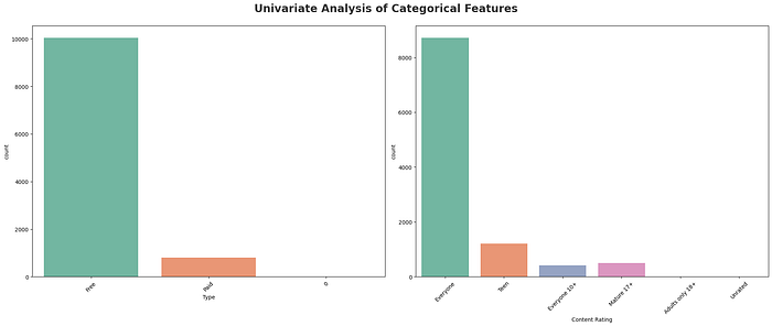

#Summary statistics and visualization of the Numeric features
plt.figure(figsize=(15, 15))
plt.suptitle('Univariate Analysis of Numerical Features', fontsize=20, fontweight='bold', alpha=0.8, y=1.0)

for i in range(0, len(numeric_features)):
    plt.subplot(5, 3, i+1)
    sns.kdeplot(x=df_copy[numeric_features[i]],shade=True, color='b')
    plt.xlabel(numeric_features[i])
    plt.tight_layout()
plt.show()

• Univariate Analysis: Analyze individual variables to understand their distribution and central tendencies.

#Identify outliers in the Rating column using box plot
plt.figure(figsize=(8, 4))
sns.boxplot(x=df_copy['Rating'], color= 'lightgreen')
plt.title('App Ratings')
plt.xlabel('')
plt.show()


#Distribution of the "Android Ver" column using countplot
order = df_copy['Android Ver'].value_counts().index #sort the values
sns.countplot(y='Android Ver', data=df_copy, order =order, palette='Set2')
plt.title('Most used Android Version')
plt.xlabel('values')
plt.ylabel('Android Version')
plt.show()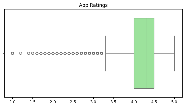

A univariate visualization of rating

A univariate visualization of Android Version

• Bivariate Analysis: Examine the relationship between two variables.

#Relationship between size of app to the rating using pairplot
sns.pairplot(df_copy[subset])
plt.show()


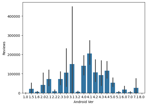
#Relationship between Android Version to the Reviews using barplot
sns.barplot(x='Android Ver', y='Reviews', data=df_copy)
plt.show()

A pairplot showing relationship between two variables

A barplot showing relationship between two variables

• Multivariate Analysis: Explore interactions among multiple variables.

#Display the correlation matrix for a subset of numerical columns
subset = ['Size', 'Rating', 'Reviews', 'Android Ver', 'Current Ver']
correlation_matrix = df_copy[subset].corr()
plt.show()
sns.heatmap(correlation_matrix, annot=True, cmap='coolwarm', fmt='.2f')
plt.show()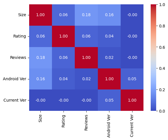

A correlation matrix showing relationship among multiple variables

PROBLEM QUESTIONS

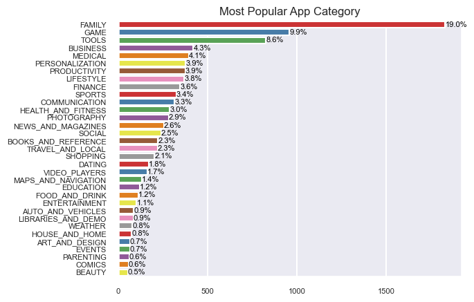
1. Which is the most popular app category?

2. Which Category has largest number of installations?

3. What are the Top 5 most installed Apps in Each popular Categories?

4. How many apps are there on Google Play Store which get 5 ratings?

# Most popular App Category
category_counts = df_copy['Category'].value_counts()
category_percentages = (category_counts / len(df_copy)) * 100
category_order = category_counts.index

# Create the count plot with category order
sns.countplot(y='Category', data=df_copy, order=category_order, palette='Set1')

# Add percentage labels to the bars
for index, value in enumerate(category_counts):
    percentage = category_percentages[index]
    plt.text(value, index, f'{percentage:.1f}%', va='center', ha='left', color='black')

# Adding title and labels
plt.title('Most Popular App Category')
plt.xlabel('')
plt.ylabel('')
plt.show()

#Category with the largest number of installation
df_cat_installs = df_copy.groupby(['Category'])['Installs'].sum().sort_values(ascending= False).reset_index()
df_cat_installs.Installs = df_cat_installs.Installs/1000000000
print(df_cat_installs.Installs)
df2 = df_cat_installs.head(10)
plt.figure(figsize = (8,6))
sns.set_context("talk")
sns.set_style("darkgrid")

ax = sns.barplot(x = 'Installs' , y = 'Category' , data = df2, color="#74B72E")
ax.set_xlabel('No. of Installations in Billions')
ax.set_ylabel('')
ax.set_title("Most Popular Categories in Play Store", size = 12)
ax.set_xticklabels(ax.get_xticklabels(), fontsize=8) 
ax.set_yticklabels(ax.get_yticklabels(), fontsize= 8)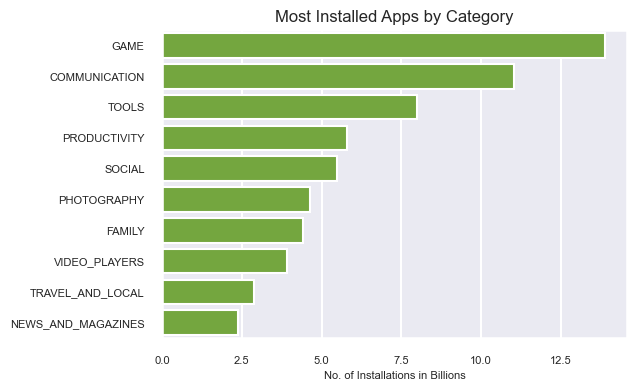

#Top 5 most installed Apps in each category
dfa = df_copy.groupby(['Category' ,'App'])['Installs'].sum().reset_index()
dfa = dfa.sort_values('Installs', ascending = False)
apps = ['GAME', 'COMMUNICATION', 'TOOLS', 'PRODUCTIVITY', 'SOCIAL' ]
sns.set_context("poster")
sns.set_style("darkgrid")

plt.figure(figsize=(40,30))

for i,app in enumerate(apps):
    df2 = dfa[dfa.Category == app]
    df3 = df2.head(5)
    plt.subplot(4,2,i+1)
    sns.barplot(data= df3,x= 'Installs' ,y='App' )
    plt.xlabel('Installation in Millions')
    plt.ylabel('')
    plt.title(app,size = 20)
    
plt.tight_layout()
plt.subplots_adjust(hspace= .3)
plt.show()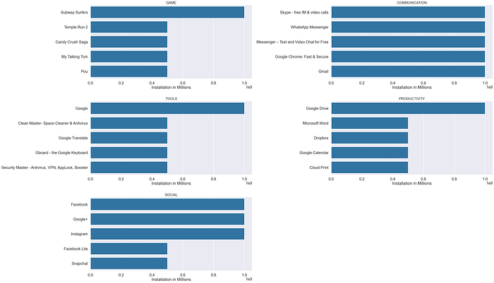

#Apps with 5 star ratings
rating = df_copy.groupby(['Category','Installs', 'App'])['Rating'].sum().sort_values(ascending = False).reset_index()
toprating_apps = rating[rating.Rating == 5.0]
print("Number of 5.0 rated apps is",toprating_apps.shape[0])
toprating_apps.head(1)

Conclusion

GooglePlayStoreAnalysis , contains the complete analysis, along with insights and observations. It serves as a comprehensive guide, walking through each step of the Exploratory Data Analysis (EDA) process.

This guide provides a deeper understanding of the dataset, and the methodologies applied in the analysis.